Introduction
The goal of this article is to explore how we can model multi-body systems using numerical techniques and simplifying assumptions. We will explore the Jupiter-Galilean Moons system to see a simple implementation of multi body orbits. In a later article, we will discuse a more accurate simulation of the system.
Simplifying Assumptions For Jupiter - Moons System and Importing Libraries
We will begin with some simplifying assumptions:
- The system is restricted to Jupiter and its Galilean moons. Small moons within the orbit of IO are not considered. The sun is not considered.
- Jupiter is initially a stationary object.
- Neglecting perturbations (Only accounting point-mass Newtonian gravity).
- Planer motion.
- No atmospheric drag.
- Each moon starts exactly at its periapsis.
import numpy as np
import matplotlib.pyplot as plt
from matplotlib.animation import FuncAnimation #can ignore
from matplotlib.patches import Circle #can ignore
import matplotlib.colors as mcolors #can ignore
Defining Constants
All constants are in SI units.
# Constants (SI units)
G = 6.67430e-11  # Gravitational constant

# Galilean moons: mass, semi-major axis, eccentricity, orbital period, and visualization color

MOONS = {
    'Io':   {'mass': 8.9319e22,
            'semi_major_axis': 421800e3,
            'eccentricity': 0.0041,
            'period': 1.769*24*3600,
            'color': 'yellow'}, #color in simulation gif
    'Europa':   {'mass': 4.7998e22,
                'semi_major_axis': 671100e3,
                'eccentricity': 0.0094,
                'period': 3.551*24*3600,
                'color': 'red'},
    'Ganymede': {'mass': 1.4819e23,
                'semi_major_axis': 1070400e3,
                'eccentricity': 0.0013,
                'period': 7.155*24*3600,
                'color': 'green'},
    'Callisto': {'mass': 1.0759e23,
                'semi_major_axis': 1882700e3,
                'eccentricity': 0.0074,
                'period': 16.69*24*3600,
                'color': 'blue'}
}

JUPITER_RADIUS = 71492e3
JUPITER_COLOR = 'orange'
M_JUPITER = 1.898e27  # Mass of Jupiter (kg)
Initial Conditions
Now we set up initial positions at periapsis using the semi-major axis and eccentricity. Velocities come from the vis-viva equation:
def initialize_system():
    positions = [np.array([0.0, 0.0])]  # Jupiter at origin
    velocities = [np.array([0.0, 0.0])]  # Jupiter initially stationary

    for moon in MOONS.values():
        a = moon['semi_major_axis']
        e = moon['eccentricity']
        r = a * (1 - e)  # periapsis distance
        pos = np.array([r, 0.0])
        v_mag = np.sqrt(G * M_JUPITER * (2/r - 1/a))
        vel = np.array([0.0, v_mag])
        positions.append(pos)
        velocities.append(vel)

    return np.array(positions), np.array(velocities)
Gravitational Acceleration
We compute pairwise gravitational acceleration for each body:
def gravitational_acceleration(positions, masses):
    n = len(positions)
    accelerations = np.zeros_like(positions)
    for i in range(n):
        for j in range(n):
            if i != j:
                r_vec = positions[j] - positions[i]
                dist_sq = np.dot(r_vec, r_vec)
                accelerations[i] += G * masses[j] * r_vec / (dist_sq *
                                    np.sqrt(dist_sq))
    return accelerations
Numerical Integration with Runge–Kutta 4
The RK4 method provides a good balance between accuracy and computational cost. We update positions and velocities every timestep . The local truncation error is on the order of while the total accumulated error is on the order of . RK4 is not symplectic, hence over a large time scale there will be an accumulation of errors. Here we have a short enough time scale where this wont cause any large issues. Our RK implementation on a high-level is: The specific steps in your implementation match the RK4 method:
- k1_v and k1_r: Initial derivatives
- k2_v and k2_r: Derivatives at halfway using k1 values
- k3_v and k3_r: Derivatives at halfway using k2 values
- k4_v and k4_r: Derivatives at the endpoint using k3 values
- Final weighted average to get the new values
def rk4_step(positions, velocities, masses, dt):
    a1 = gravitational_acceleration(positions, masses)
    k1_v = a1 * dt; k1_r = velocities * dt

    a2 = gravitational_acceleration(positions + 0.5*k1_r, masses)
    k2_v = a2 * dt; k2_r = (velocities + 0.5*k1_v) * dt

    a3 = gravitational_acceleration(positions + 0.5*k2_r, masses)
    k3_v = a3 * dt; k3_r = (velocities + 0.5*k2_v) * dt

    a4 = gravitational_acceleration(positions + k3_r, masses)
    k4_v = a4 * dt; k4_r = (velocities + k3_v) * dt

    positions_new = positions + (k1_r + 2*k2_r + 2*k3_r + k4_r)/6
    velocities_new = velocities + (k1_v + 2*k2_v + 2*k3_v + k4_v)/6
    return positions_new, velocities_new
Running the Simulation
We integrate for one Jovian month (~30.44 days) mapped to a 60-second animation. This cell runs the core loop and stores trajectories.
def run_simulation(duration, dt):
    positions, velocities = initialize_system()
    masses = np.array([M_JUPITER] + [m['mass'] for m in MOONS.values()])
    steps = int(duration / dt)
    traj = np.zeros((steps, len(masses), 2))
    traj[0] = positions

    for i in range(1, steps):
        positions, velocities = rk4_step(positions, velocities, masses, dt)
        traj[i] = positions
        if i % (steps // 10) == 0:
            print(f"Progress: {i/steps:.1%}")
    return traj

# Example usage
sim_duration = 30.44 * 24*3600  # seconds
real_time = 60  # seconds of animation
fps = 30
dt = sim_duration / (real_time * fps)
trajectory = run_simulation(sim_duration, dt)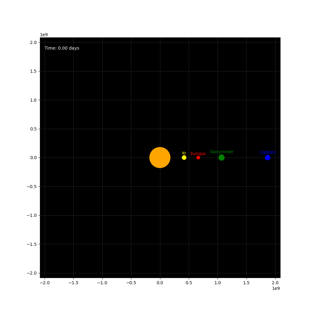
Citations
- Newman, M. E. J. (2013). Computational physics. Createspace.
- Galilean moons of Jupiter. Nasa.gov. (2013, July). https://www.nasa.gov/wp-content/uploads/2009/12/moons_of_jupiter_lithograph.pdf