From Diffusion to Fractional Diffusion: A CTRW Approach to Anomalous Transport
April 16, 2026
The standard diffusion equation assumes a finite mean waiting time and a finite jump variance. When either assumption fails, as it does for tracer particles in turbulent plasmas with long trapping events and large radial jumps, the central limit theorem no longer applies and the diffusion equation is replaced by a fractional diffusion equation derived from a heavy-tailed continuous-time random walk.
Since the earliest tokamak experiments, measured cross-field transport has exceeded both classical and neoclassical predictions, often by one to two orders of magnitude [3, 4]. The standard picture attributes this to turbulence. There is also a mathematical issue. The local diffusive model for a scalar field ϕ,
∂tϕ=∂x[χ∂xϕ]+S,
follows from a conservation law and Fick’s law. Its derivation from a Brownian random walk requires Gaussian statistics, Markovian dynamics, and a well-defined transport scale [1]. Turbulent trapping and large radial flights violate all three.
We ask what equation replaces ordinary diffusion when the underlying stochastic process has heavy-tailed statistics. One such equation, developed by Montroll and Weiss [5], Metzler and Klafter [1], and others, is a fractional diffusion equation
0CDtβP=χD∣x∣αP,
where 0CDtβ is the Caputo fractional time derivative of order 0<β≤1, and D∣x∣α is the Riesz fractional space derivative of order 0<α≤2. For α=2 and β=1 the equation reduces to the ordinary diffusion equation. The fractional orders are set by the tail exponents of the jump and waiting-time distributions in the underlying CTRW.
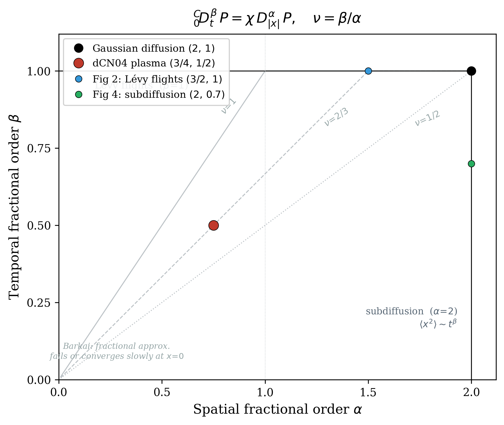
Parameter space of the fractional diffusion equation [eq:fde] in the (α, β) plane. The spatial order α controls the tail decay of the propagator (P ∼ |x|−(1 + α)), while the temporal order β controls memory. Ordinary Gaussian diffusion sits at (α, β) = (2, 1). The right edge α = 2 with β < 1 gives subdiffusion with ⟨x2⟩ ∼ tβ; the top edge β = 1 with α < 2 gives Markovian Lévy flights. Dashed contours show the similarity exponent ν = β/α, which determines the self-similar scaling of the Green’s function. The plasma-turbulence parameters of del-Castillo-Negrete et al.[2], (α, β) = (3/4, 1/2) with ν = 2/3, are marked alongside the simulation parameters used in Figures 3 and 5. Near the lower-left corner, convergence of the fractional approximation to the exact CTRW becomes slow, especially at x = 0[6].
An application to plasma turbulence was given by del-Castillo-Negrete, Carreras, and Lynch [2, 7]. They simulated tracer particles in pressure-gradient-driven plasma turbulence and found that the radial displacement pdf had algebraic tails decaying as ∣x∣−(1+α) with α≈3/4, and that the similarity exponent was ν=2/3. Equation [eq:fde] with α=3/4 and β=1/2 reproduced these results quantitatively.
The thesis is organized as follows. Section 2 derives the fractional diffusion equation from the CTRW, treating the Brownian and heavy-tailed cases side by side. Section 3 defines the fractional operators and shows how they invert the Fourier-Laplace transform of the CTRW solution. Section 4 discusses the physical content of the model and its limitations.
From Random Walks to Fractional Diffusion
The Montroll—Weiss Equation
Consider a particle that waits a random time τi drawn from a pdf ψ(τ), then jumps by a random displacement ζi drawn from a pdf λ(ζ). We assume waiting times and jump lengths are independent. The probability P(x,t) of finding the particle at position x at time t satisfies the Montroll—Weiss equation [1]:
The first term accounts for particles that have not yet jumped. The second accounts for particles that arrived at x′ at time t′ and then jumped to x. Introducing the Fourier transform f^(k)=∫eikxf(x)dx and the Laplace transform f~(s)=∫0∞e−stf(t)dt, equation [eq:MW_real] becomes algebraic [1]:
P~^(k,s)=s1−ψ~(s)⋅1−ψ~(s)λ^(k)1.
Apply the Laplace transform to [eq:MW_real]. The survival probability ∫t∞ψ(t′)dt′ in the first term has Laplace transform
where Fubini’s theorem was used to exchange the order of integration. The second term in [eq:MW_real] is a time convolution of ψ with the spatial convolution ∫λ(x−x′)P(x′,t′)dx′. By the Laplace convolution theorem it transforms to ψ~(s) times the Laplace transform of the spatial term; the Fourier convolution theorem then converts the spatial integral to λ^(k)P~^(k,s). Taking the Fourier transform of the first term gives δ^(k)⋅(1−ψ~(s))/s=(1−ψ~(s))/s. Assembling both sides:
Take an exponential waiting-time pdf ψM(τ)=μe−μτ with finite mean ⟨τ⟩=1/μ, and a Gaussian jump pdf λF(ζ)=(2πσ)−1/2exp(−ζ2/2σ) with finite variance ⟨ζ2⟩=σ. To take the continuum limit, we rescale waiting times by a factor r and jumps by a factor h, then send r,h→0. The small-parameter expansions of the transforms are
Substituting [eq:psi_gauss]—[eq:lam_gauss] into [eq:MW] and expanding to leading order in r and h, the numerator becomes 1−ψ~(rs)≈rs⟨τ⟩, while the denominator factor satisfies
where the cross-term rs⟨τ⟩⋅21⟨ζ2⟩h2k2 is of higher order in r and h and is dropped. To see this consistently: the diffusivity χ=h2⟨ζ2⟩/(2r⟨τ⟩) is held finite as r,h→0, which requires h2∼r. Under this coupling the cross-term scales as r⋅h2∼r2, while the two retained terms each scale as r, so the cross-term is sub-leading and the truncation is self-consistent. Therefore
where χ=h2⟨ζ2⟩/(2r⟨τ⟩) is held finite as r,h→0. Rearranging gives
sP~^−1=−χk2P~^.
Using P(x,0)=δ(x), the standard transform identities
L[∂tP]F[∂x2P]=sP~(s)−δ(x),=−k2P^(k),
invert [eq:diff_FL] to give ∂tP=χ∂x2P. This holds whenever both ⟨τ⟩ and ⟨ζ2⟩ are finite [1].
Heavy Tails and the Breakdown of the CLT
Now suppose the dynamics produces power-law tails [2]:
ψ(τ)∼τ−(1+β),0<β<1,λ(ζ)∼∣ζ∣−(1+α),0<α<2.
The mean waiting time ⟨τ⟩=∫τψ(τ)dτ diverges because β<1. The jump variance ⟨ζ2⟩=∫ζ2λ(ζ)dζ diverges because α<2. More generally, the moment ⟨∣ζ∣n⟩ diverges for any n≥α [1]. Neither ⟨τ⟩ nor ⟨ζ2⟩ exists, so the standard CLT does not apply and the continuum limit cannot produce the ordinary diffusion equation.
What happens instead is governed by a Tauberian theorem: a pdf with algebraic tail ψ(τ)∼τ−(1+β) has a Laplace transform that behaves, for small s, as ψ~(s)≈1−c1sβ. The singularity structure of the transform at small argument encodes the slow decay of the pdf at large argument. Similarly, λ^(k)≈1−c2∣k∣α for small k [1]. Rescaling as before and substituting into [eq:MW]:
again dropping the higher-order cross-term. Assembling:
P~^≈s(c1rβsβ+c2hα∣k∣α)c1rβsβ=sβ+χ∣k∣αsβ−1,
where χ=c2hα/(c1rβ) is held finite. To obtain a nontrivial continuum limit, the two denominator terms must remain of the same order as r,h→0. This scaling keeps the spatial and temporal terms at the same order in the continuum limit. Rearranging gives
sβP~^−sβ−1=−χ∣k∣αP~^.
Compare this with [eq:diff_FL]: s has been replaced by sβ, and k2 by ∣k∣α. The tail exponents of the underlying random walk now appear as the orders of the operators in transform space. The next question is which real-space operators correspond to sβ and ∣k∣α.
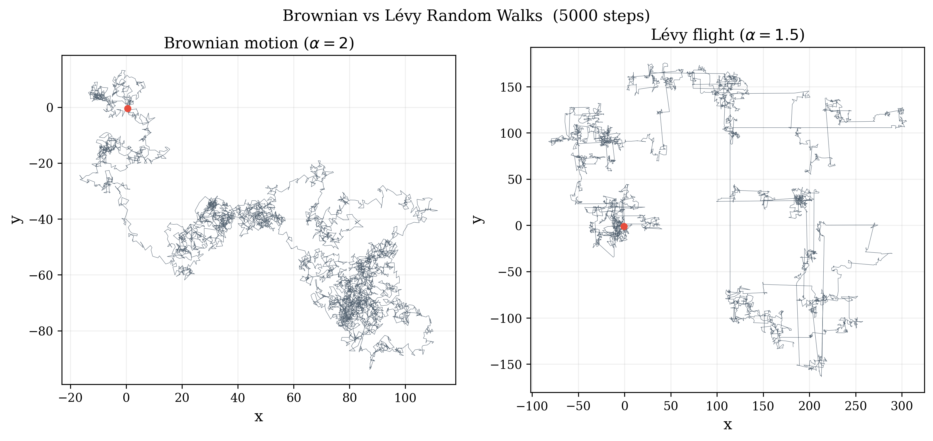
Brownian walk (α = 2, Gaussian jumps, 5000 steps) versus Lévy flight (α = 1.5, heavy-tailed jumps, 5000 steps). The Brownian path fills space more or less uniformly, consistent with a finite jump variance and Gaussian propagator. The Lévy path illustrates the effect of the heavy-tailed jump distribution in [eq:heavy_tails]: local motion interrupted by occasional long flights.
Fractional Operators and the Fractional Diffusion Equation
The Riemann—Liouville Fractional Integral and Derivative
The fractional integral is a generalization of the Cauchy formula for repeated integration. For integer n, the n-fold integral of ϕ from a to x can be written as a single convolution integral [1]:
aDx−nϕ=(n−1)!1∫ax(x−y)n−1ϕ(y)dy.
Replacing (n−1)! with Γ(ν) extends this to non-integer order ν>0:
aDx−νϕ=Γ(ν)1∫ax(x−y)ν−1ϕ(y)dy.
The Riemann—Liouville fractional derivative of order α is then defined as an integer differentiation of a fractional integral [2]:
aDxαϕ=dxmdm[aDx−(m−α)ϕ],m=⌈α⌉,
where m is the smallest integer greater than α. For 1<α≤2, we have m=2 and the derivative takes the explicit form
aDxαϕ=Γ(2−α)1∂x2∫ax(x−y)α−1ϕ(y)dy.
For 0<α≤1, one has m=1 and the second derivative above is replaced by a first derivative. In either case the operator is non-local: it depends on the values of ϕ over the entire interval (a,x), not just at x.
Example 1. The RL derivative of a power function with a=0: 0Dxμxλ=Γ(λ−μ+1)Γ(λ+1)xλ−μ, which reduces to the ordinary derivative for integer μ.
A key property for Fourier analysis: on the semi-infinite domain (−∞,x), the Weyl fractional derivative satisfies −∞Dxμeikx=(ik)μeikx [1].
Left, Right, and Symmetric Derivatives
The RL derivative [eq:RL_deriv] integrates to the left of x. A right derivative, integrating over (x,b), is defined analogously [2]:
xDbαϕ=Γ(m−α)(−1)m∂xm∫xb(y−x)α+1−mϕ(y)dy.
The general spatial fractional operator is a weighted sum Dxα=w−aDxα+w+xDbα, where w± control left-right asymmetry. The symmetric Riesz derivative on (−∞,∞) is defined as [2]:
D∣x∣α=2cos(πα/2)−1[−∞Dxα+xD∞α],
and its Fourier transform, for 0<α<2, gives
F[D∣x∣αϕ]=−∣k∣αϕ^(k,t).
To derive [eq:riesz_FT], apply the Fourier transform directly using the Weyl eigenvalue relations −∞Dxαeikx=(ik)αeikx and xD∞αeikx=(−ik)αeikx [1]. For any real k, writing ik=∣k∣ei(π/2)sgn(k) and −ik=∣k∣e−i(π/2)sgn(k), one has
confirming [eq:riesz_FT]. The prefactor −1/(2cos(πα/2)) in the definition of the Riesz operator is the constant needed to cancel the cosine and yield the Fourier symbol −∣k∣α. This holds for the full range 0<α<2, which is important because the plasma case study of del-Castillo-Negrete et al. uses α=3/4<1.
The Caputo Time Derivative
For the time direction, the RL time derivative has the Laplace transform L, which involves the initial value of a fractional integral of ϕ rather than ϕ itself. This is not suitable for initial-value problems. The Caputo derivative resolves this by switching the order of differentiation and integration [2]:
0CDtβϕ=Γ(1−β)1∫0t(t−τ)β∂τϕ(x,τ)dτ,0<β<1.
Its Laplace transform is
L[0CDtβϕ]=sβϕ~(s)−sβ−1ϕ(0),
To derive [eq:caputo_LT], write the Caputo derivative [eq:caputo] as the time convolution 0CDtβϕ=(∂tϕ)∗g where g(t)=t−β/Γ(1−β). By the Laplace convolution theorem,
L[0CDtβϕ]=L[∂tϕ]⋅L[g].
The first factor is L[∂tϕ]=sϕ~(s)−ϕ(0). For the second, the substitution u=st gives
L[t−β]=∫0∞e−stt−βdt=sβ−1∫0∞e−uu−βdu=Γ(1−β)sβ−1,
so L[g]=sβ−1. Combining and expanding:
L[0CDtβϕ]=sβ−1(sϕ~(s)−ϕ(0))=sβϕ~(s)−sβ−1ϕ(0),
which is [eq:caputo_LT], and depends directly on ϕ(0). The Caputo derivative of a constant is zero, unlike the RL derivative. This is necessary for well-defined steady-state solutions.
Assembling the Equation
We had from the CTRW continuum limit, equation [eq:fde_FL]:
sβP~^−sβ−1=−χ∣k∣αP~^.
From [eq:caputo_LT], the left side is the Fourier-Laplace transform of 0CDtβP with P(x,0)=δ(x). From [eq:riesz_FT], the right side is χ times the transform of D∣x∣αP. Inverting:
0CDtβP=χD∣x∣αP.
This is the fractional diffusion equation. At α=2, β=1 the Caputo derivative reduces to ∂t and the Riesz derivative to ∂x2, recovering ordinary diffusion.
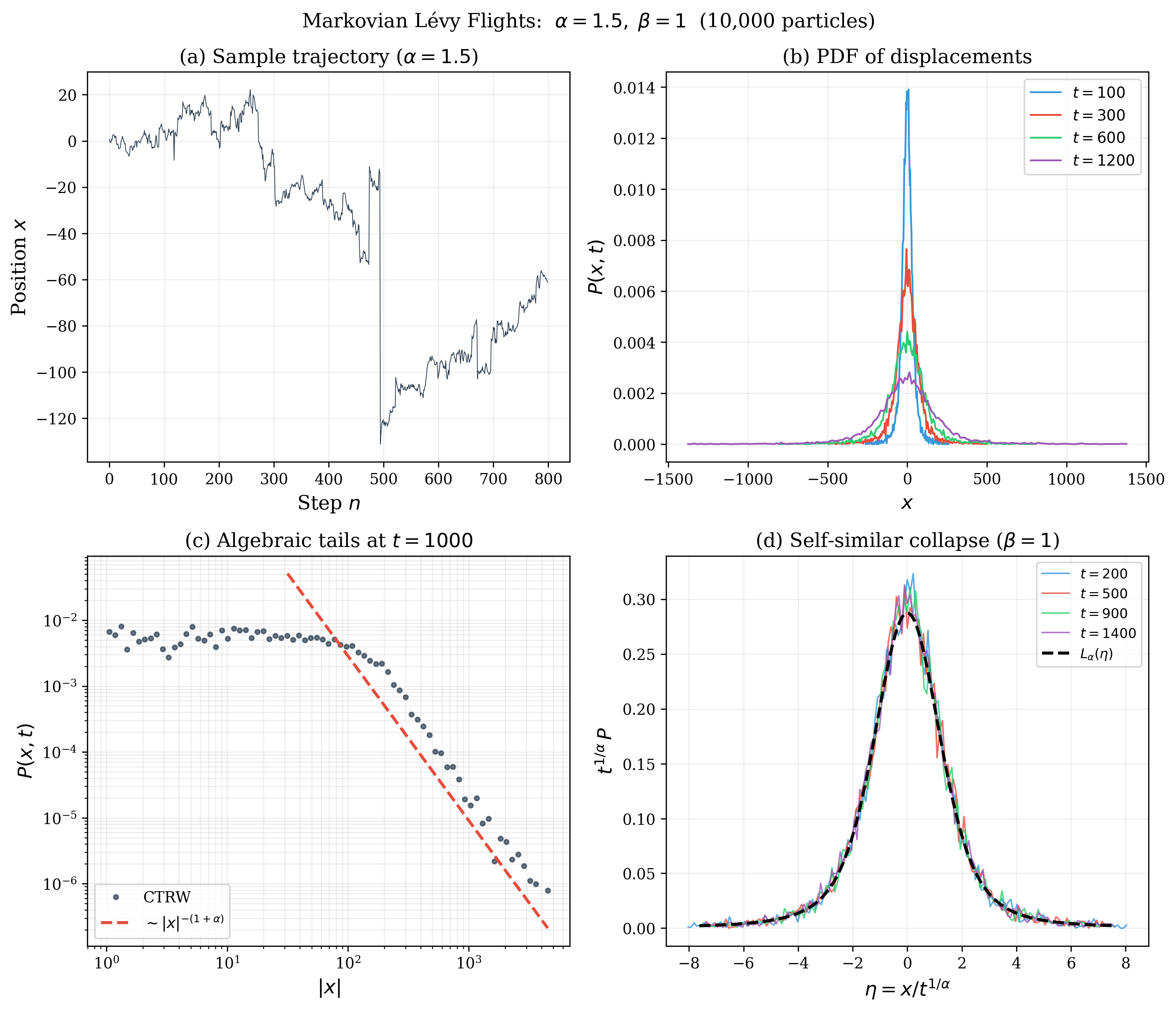
CTRW simulation with α = 1.5, β = 1 (Markovian Lévy flights, 10,000 particles). (a) A single trajectory showing local motion interrupted by long flights. (b) The pdf of particle displacements broadens with time but remains non-Gaussian. (c) The tails of the pdf at t = 1000, plotted on log-log axes, are consistent with the algebraic decay P ∼ |x|−(1 + α) predicted by the fractional Green’s function [eq:tail_decay]. (d) Self-similar collapse: when each pdf is rescaled by t1/α and plotted against η = x/t1/α, the curves collapse closely onto the analytical α-stable density Lα(η) (black dashed line). This is consistent with the large-scale limit described by [eq:fde_final].
Properties of the Solution
The Fourier—Laplace transform of [eq:fde_final], with initial condition G(x,0)=δ(x) so that G^(k,0)=1, is precisely [eq:fde_FL]. Solving algebraically for G~^:
G~^(k,s)=sβ+χ∣k∣αsβ−1.
Inverting the Laplace transform uses the Mittag-Leffler identity L[Eβ(−ctβ)]=sβ−1/(sβ+c), which follows from the series Eβ(−ctβ)=∑n=0∞(−c)ntβn/Γ(βn+1) and the standard transform L[tβn]=Γ(βn+1)/sβn+1:
For the parameter choice used here, α>β, and the corresponding Green’s function is a proper probability density [2]; in the plasma case, α=3/4>β=1/2. The self-similar form of the Green’s function of [eq:fde_final] now follows. To see the scaling explicitly, suppose G(x,t)=t−νK(x/tν) for some exponent ν and profile K. Substituting into the Fourier transform and changing variables η=x/tν gives G^(k,t)=K^(ktν). For this to equal Eβ(−χ∣k∣αtβ) from [eq:green_Fourier], the argument ktν must absorb all t-dependence; this requires ∣ktν∣α∝∣k∣αtβ, which forces να=β, i.e. ν=β/α. The full scaling factor follows from normalisation ∫Gdx=1. Since G^ depends on k and t only through the combination χ∣k∣αtβ=∣k(χ1/βt)β/α∣α, the inverse Fourier transform must satisfy G(x,t)=(χ1/βt)−β/αK(η) with similarity variable
G(x,t)=(χ1/βt)−β/αK(η),η=x(χ1/βt)−β/α,
where the profile K is the inverse Fourier transform of K^(q)=Eβ(−∣q∣α), i.e., K(η)=(1/π)∫0∞cos(ηz)Eβ(−zα)dz [2]. Two asymptotic regimes characterize K: near the origin, K(η)∼A/η1−α+B (a weak cusp for α<1), and for large ∣η∣,
K(η)∼η1+αC,C=π1Γ(1+β)Γ(1+α)sin2πα.
The large-∣η∣ tail of K follows from the small-∣q∣ behaviour of K^. Using the power-series definition
Eβ(−z)=n=0∑∞Γ(βn+1)(−z)n,
we obtain, for small z,
Eβ(−z)=1−Γ(1+β)z+O(z2).
Substituting z=∣q∣α gives
K^(q)=Eβ(−∣q∣α)=1−Γ(1+β)∣q∣α+O(∣q∣2α),
so the leading non-analytic term is −∣q∣α/Γ(1+β). The Tauberian theorem for Fourier transforms [1] states that a function whose Fourier transform behaves as −A∣q∣α near q=0 has algebraic tails AΓ(1+α)sin(πα/2)/(π∣η∣1+α); setting A=1/Γ(1+β) gives C=Γ(1+α)sin(πα/2)/(πΓ(1+β)), confirming [eq:tail_decay].
An important caveat concerns the moments. Formally, the n-th moment of the self-similar propagator scales as
⟨∣x∣n⟩∼tnβ/α,
so the similarity exponent ν=β/α determines the transport regime: ν=1/2 for ordinary diffusion, ν>1/2 for superdiffusion, ν<1/2 for subdiffusion. However, because K(η)∼η−(1+α) for large η, the integrand ηnK(η)∼ηn−1−α diverges for n≥α when integrated over (−∞,∞) [2]. In particular, for α<2 the mean squared displacement is not defined on the infinite line. Del-Castillo-Negrete et al. handle this by introducing a finite spatial cutoff, which is physically natural since real systems always have a bounded domain [2]. The moments that do remain well-defined are the fractional moments ⟨∣x∣δ⟩ for δ<α, which are finite and scale as tδβ/α.
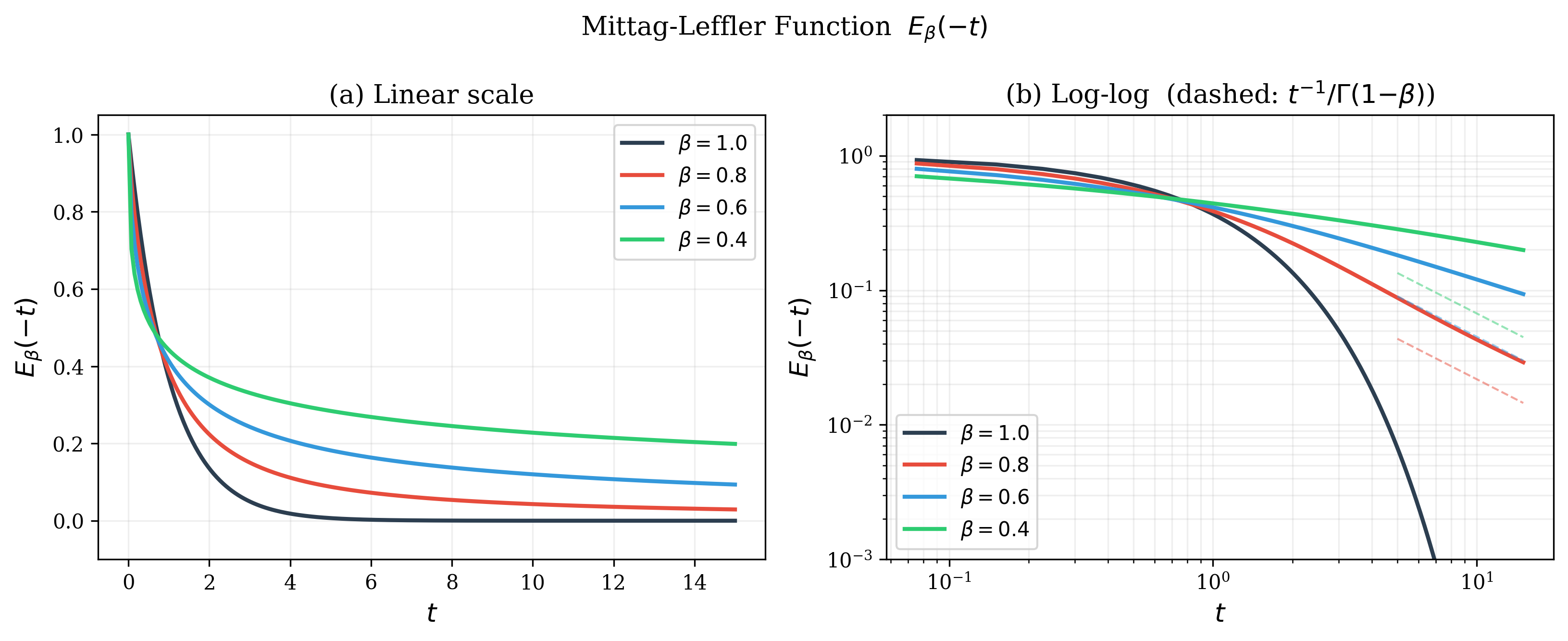
The Mittag-Leffler function Eβ(−t) for several values of β, computed via integral representation. For β = 1 it reduces to e−t (exponential decay). For β < 1 it decays algebraically as ∼ t−1/Γ(1 − β) at large t (dashed lines), rather than exponentially. This is the temporal analogue of the heavy spatial tails in [eq:tail_decay]: both arise from the non-Markovian memory encoded by the Caputo fractional time derivative. The Mittag-Leffler function also appears in the Green’s function through [eq:green].
Discussion and Conclusion
The Plasma Case Study
Del-Castillo-Negrete et al. [2] simulated 25,000 tracer particles in 3D resistive pressure-gradient-driven turbulence. The turbulence produces E×B eddies that trap particles, and avalanche-like instabilities that launch them on long radial flights. Both effects are visible in the tracer orbits (their Figure 2). The measured pdf of radial displacements has tails decaying as ∣x∣−1.75, giving α≈3/4. The similarity exponent, measured from the collapse of the pdf under rescaling by tν, is ν≈2/3, which with ν=β/α requires β=1/2. With χ=0.09, the fractional model [eq:fde_final] reproduces both the pdf shape and the self-similar collapse. Note that because α=3/4<1, the mean squared displacement of the fractional Green’s function is not finite on the full line, and the moment scaling reported in [2] relies on the finite spatial extent of the simulation domain acting as a natural cutoff.
This case is interesting because α<1 places it outside the regime where the RL derivative takes the more familiar m=2 form [eq:RL_explicit]. The Riesz derivative is still well-defined for this value through its Fourier transform property [eq:riesz_FT], and the derivation from the CTRW in Section 2 does not require α>1.
The subdiffusion case α=2, β<1 visible in Figure 5 (right column) is worth isolating, as it clarifies the role of the temporal fractional order in the absence of any spatial anomaly. Setting α=2 in [eq:fde_final] gives 0CDtβP=χ∂x2P: the spatial operator is the ordinary Laplacian, but the Caputo time derivative introduces non-Markovian memory through the convolution in [eq:caputo]. The Green’s function [eq:green] reduces to G(x,t)=t−β/2K(η) with η=x/tβ/2, and the MSD grows as ⟨x2⟩∼tβ<t for β<1, that is, slower than ordinary diffusion. The connection to Figure 4 is direct: the Fourier transform G^(k,t)=Eβ(−χk2tβ) decays as a Mittag-Leffler function in time at fixed k. At large t, the asymptotic Eβ(−χk2tβ)∼(χk2tβ)−1/Γ(1−β) corresponds to the algebraic relaxation visible in Figure 4 for β<1. The slowdown arises entirely from the divergent mean waiting time ⟨τ⟩: the spatial jump distribution remains Gaussian, and only the waiting-time distribution is anomalous.
Three transport regimes simulated via CTRW. Top row: pdfs at a fixed time, with analytical curves overlaid where available. Bottom row: moment scaling on log-log axes. Left column: normal diffusion (α = 2, β = 1), with Gaussian pdf and linear MSD scaling ⟨x2⟩ ∼ t. Centre column: Lévy flights (α = 1.5, β = 1), where the MSD diverges and instead the fractional moment ⟨|x|1.0⟩ is plotted (since 1.0 < α = 1.5, this moment is finite), scaling as tδ/α = t0.67. Right column: subdiffusion (α = 2, β = 0.7), where the MSD is finite but grows sublinearly as t0.7. All three regimes are described by [eq:fde_final] with different (α, β).
Connection to Experimental Diagnostics
Transfer-entropy studies have also been discussed in CTRW language. Van Milligen et al. [8] describe “slow” and “fast” transport channels, with the latter consistent with jump-like propagation across minor transport barriers. This is qualitatively compatible with a heavy-tailed jump distribution, but it is not a derivation of the fractional model.
The NLCC method of Ding et al. [9] addresses a different question: directional asymmetry in nonlinear coupling between radially separated probe signals. Such asymmetry may be compared with an imbalance between left and right spatial fractional derivatives, but I did not find such a connection in the literature. The NLCC construction itself is based on phase-space reconstruction rather than fractional calculus.
They are discussed further in the author’s physics thesis.
Limitations of the Fractional Approximation
The fractional diffusion equation is an asymptotic result: it describes the large-scale, long-time behaviour of the CTRW, and can converge slowly at finite times or near the origin. Barkai [6] showed that the exact CTRW propagator at x=0 may differ from the fractional Green’s function over a long transient, because the fractional equation captures only the leading term of the asymptotic expansions [eq:psi_heavy]—[eq:lam_heavy]. Higher-order corrections in s and k are discarded in taking the continuum limit, and these corrections matter most near the origin and at early times.
Separately, Rodriguez-Fernandez et al. [10] showed that cold-pulse phenomena in tokamaks, which have been cited as evidence of nonlocal transport, can be reproduced by local quasilinear turbulent transport models (specifically the TGLF-SAT1 saturation rule). This does not invalidate the fractional framework, but it does mean that apparently nonlocal transport signatures in experiments are not by themselves enough to establish genuinely nonlocal transport. The fractional model is a reduced model: it compactly captures certain statistical features of anomalous transport, not the underlying first-principles dynamics.
Conclusion
We derived the fractional diffusion equation from the CTRW by showing that heavy-tailed jump and waiting-time distributions produce, in the continuum limit, transform-space operators ∣k∣α and sβ that correspond to the Riesz and Caputo fractional derivatives respectively. The fractional orders are not free parameters: they are fixed by the tail exponents of the underlying stochastic process. The plasma-turbulence results of del-Castillo-Negrete et al. provide a case where this framework is tested against simulation data, and the CTRW simulations presented here reproduce the main qualitative signatures: algebraic tails, self-similar collapse, and, for moments of order below α, anomalous scaling. The natural extension is to bounded domains, where the truncated RL derivatives become singular at the boundaries and require Caputo-style regularization [11]. That problem is directly relevant to radial transport modelling in confined plasmas.
[8] B. Van Milligen, B. Carreras, L. García, and J. Nicolau, “The Radial Propagation of Heat in Strongly Driven Non-Equilibrium Fusion Plasmas,” Entropy, 21, no. 2, 148 (2019), doi:10.3390/e21020148, https://www.mdpi.com/1099-4300/21/2/148.
[10] P. Rodriguez-Fernandez, A. E. White, N. T. Howard, B. A. Grierson, G. M. Staebler, J. E. Rice, X. Yuan, N. M. Cao, A. J. Creely, M. J. Greenwald, A. E. Hubbard, J. W. Hughes, J. H. Irby, and F. Sciortino, “Explaining Cold-Pulse Dynamics in Tokamak Plasmas Using Local Turbulent Transport Models,” Physical Review Letters, 120, no. 7, 075001 (2018), doi:10.1103/PhysRevLett.120.075001, https://link.aps.org/doi/10.1103/PhysRevLett.120.075001.