Notes: Monte Carlo Methods in Financial Engineering

Since MC method uses random sampling from unifrom distributions, on some runs of the code above, n=10 may be more accurate than n=100 for the function x^2! This seems to happen less with the function sin(x).

Variance and Asymptotic Normality

We define the variance of the function $f$ over the interval $[0,1]$ as:

Since $\alpha = \mathbb{E}[f(U)]$, we are interested in the variance of the random variable $f(U)$, where $U \sim \text{Uniform}(0,1)$.

By the standard formula for variance:

This is equivalent to:

which expresses the same variance as a mean squared deviation from $\alpha$. ²

def sigma_squared(func, n):
    '''
    This function estimates the variance of the function func over the interval [0, 1].    
    '''
    alpha = exact_integral
    return integrate.quad(lambda x: (func(x) - alpha)**2, 0, 1)[0]

print("Variance of f(x) = sin(x) over [0, 1]:", sigma_squared(f_x, 10000))

Variance of f(x) = sin(x) over [0, 1]: 0.0613536733034302

Now consider the Monte Carlo estimate:

Because the $U_i$ are i.i.d., the values $f(U_i)$ are also i.i.d. with mean $\alpha$ and variance $\sigma^2_f$.
Therefore, the variance of the sample mean is:

By the central limit theorem, as $n \to \infty$, the sampling distribution of $\hat{\alpha}_n$ becomes approximately normal:

This implies that the error term

is approximately normally distributed with:

• Mean: $0$
• Standard deviation: $\sigma_f / \sqrt{n}$

def error_term(func,mc_estimator,exact_integral,n):
    return  mc_estimator(func,n) - exact_integral

n = 1000
errorsList =[error_term(f_x,monte_carlo_integrator,  exact_integral, n) for _ in range(1000)]
plt.xlabel('Error: alpha_hat - alpha')
plt.ylabel('Frequency of Error')
plt.title('Histogram of Errors in Monte Carlo Integration Demonstrating Central Limit Theorem')
plt.hist(errorsList, bins=30, density=True, alpha=0.6, color='r')
plt.savefig('histogram_MC_Integration_CLT.png', transparent=True)
plt.show()

print(f"Mean of errors: {np.mean(errorsList):.6f}")
print(f"Standard deviation of errors: {np.std(errorsList):.6f}")
print(f"Theoretical Standard Deviation: {math.sqrt(sigma_squared(f_x, n) / n):.6f}")

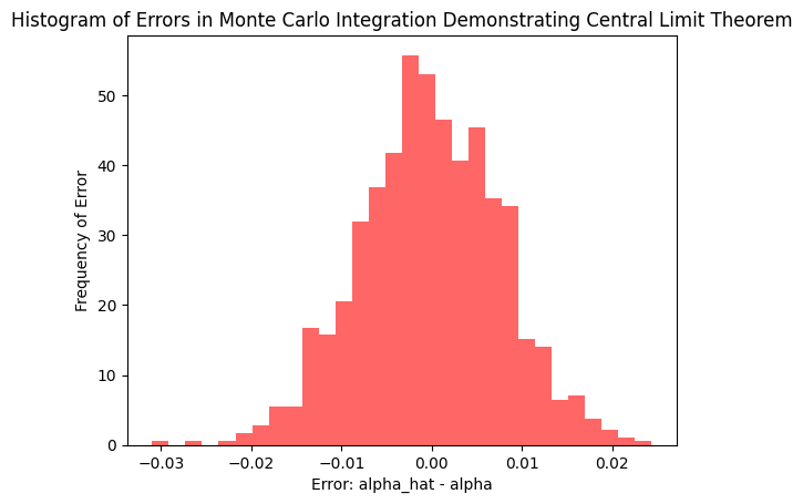
Mean of errors: -0.000182
Standard deviation of errors: 0.007798
Theoretical Standard Deviation: 0.007833

In practice, $\sigma^2_f$ is usually unknown because it depends on the unknown integral $\alpha$.
We approximate it using the sample variance of the observed values $f(U_1), \dots, f(U_n)$:

and the sample standard deviation is:

This gives us a way to estimate the uncertainty in the Monte Carlo approximation.

def sample_standard_deviation(func, n, monte_carlo_integrator):
    '''
    Calculate sample standard deviation using the formula from page 2.
    '''
    # Generate n samples
    samples = [random.uniform(0, 1) for _ in range(n)]
    
    # Calculate f(U_i) values
    f_values = [func(u) for u in samples]
    
    alpha_hat = monte_carlo_integrator(func, n)
    
    squared_deviations = [(f_val - alpha_hat)**2 for f_val in f_values]
    s_f = math.sqrt(sum(squared_deviations) / (n - 1))
    
    return s_f

n=1000
print(f"Sample Standard Deviation: {sample_standard_deviation(f_x, n, monte_carlo_integrator)/ math.sqrt(n):.6f}")    

Sample Standard Deviation: 0.007941

Why Monte Carlo?

For 1-dimensional twice-differentiable functions, the trapezoidal rule’s error rate is $O(n^{-2})$ while the MC method’s error rate is $O(n^{-1/2})$. Hence, for low-dimensional integrals the MC method is not competitive.

MC method truely shines on larger dimensional integrals as the error rate stays $O(n^{-1/2})$ while the trapezoidal rule has error rate $O(n^{-2/d})$ (it decays with higher dimensions).

Modeling the value of a derivative secruity using MC requires simulating multiple stochastic paths (say, with Geometric Brownian Motion) that model the evolution of the underlying security, interest rates, model parameters, and other relevant factors. Instead of sampling from $[0,1]^d$, we sample from a space of paths (which are all possible trajectories of the price of the underlying security). As stated in the textbook: “The dimension will ordinarily be at least as large as the number of time steps in the simulation, and this could easily be large enough to make the square-root convergence rate for Monte Carlo competitive with alternative methods.”

1.1.2 First Examples

• $S(t)$: Price of the stock at time $t$.
• $K$: Strike price; the fixed price at which the holder can buy the stock.
• $T$: Expiry time; the fixed future time at which the option can be exercised.
• $t$: Current time

Call option — A financial contract granting the right (not obligation) to buy a stock at price $K$ at time $T$.³

The payoff to the holder at time $t=T$ is:

If $S(T) > K$, the option is exercised, and the holder profits: $S(T) - K$. If $S(T) \leq K$, the option expires worthless (no profit or loss).

We multiply by a discount factor $e^{-rt}$, where r is a continuously compound interest rate. The expected present value is defined as $\mathbb{E}[e^{-rt}(S(T) - K)^+]$.

• Note: This discount factor should feel familiar to any physicist. This is the same decay factor used in damped springs and radioactive decay. Its form comes from solving differential equations of the form $\frac{dy}{dt} = ky$. Discount factor is applied due to money being compounded with a factor of $e^{rt}$. i.e If you have $V$ dollars today, you could invest it risk-free and have $Ve^{rT}$ dollars at time $T$.

To describe the evolution of the stock prices we employ the Black-Scholes equation, a stochastic differential equation.

• $\sigma$ is the volatility of the price of the underlying security.
• $r$ is the mean rate of return $\equiv$ interest rate (through some measure theory (change in metric) I don’t quite understand). This equivalance implies risk-neutral dynamics.
• $W$ is standard Brownian motion.

We can interpret this by saying we find the percentage changes ($dS/S$) as increments of Brownian motion.

The solution the SDE is:

at terminal time $T$. W is normally distributed with mean $0$ and variance $T$ - which is the same as the distribution of $\sqrt{T}Z$ where $Z \sim N(0,1)$.

S0 = 100    # S(0)
r = 0.05    # risk-free rate  
sigma = 0.2 # volatility
T = 1.0     # time to expiration
n_scenarios = 10000

def S_T (S0,r,sigma,T,n_scenarios):
    # Generate n scenerios
    # W(T) = sqrt(T) * Z, Z ~ N(0,1)
    Z = np.random.normal(0, 1, n_scenarios)
    W_T = np.sqrt(T) * Z

    #Exact Soultion
    S_T = S0 * np.exp((r - 0.5*sigma**2)*T + sigma*W_T)
    
    return S_T

#Visualization
plt.hist(S_T (S0,r,sigma,T,n_scenarios), bins=50, density=True, alpha=0.7, color='skyblue')
plt.xlabel('Stock Price at T=1')
plt.ylabel('Probability Density')
plt.title('Lognormal Distribution of Stock Prices at T=1')
plt.savefig('lognormal_distribution.png', transparent=True)
plt.show()

print(f"Theoretical mean: {S0 * np.exp(r*T):.2f}")
print(f"Simulated mean: {np.mean(S_T):.2f}")

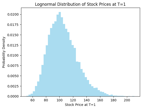
Theoretical mean: 105.13
Simulated mean: 105.13