Nonlinear Cross-Correlation Analysis of Plasma Turbulence

Introduction

Cross-field transport in magnetically confined plasmas often exceeds classical and neoclassical estimates by a large margin. This is usually attributed to turbulence and remains one of the central problems in magnetic confinement [3]. A simple starting point is the transport balance

$$\partial_t f = -\partial_r q + S,$$

where $f$ is a transported scalar, $q$ is the radial flux, and $S$ is a source term. In a local diffusive model one writes

$$q = -D\,\partial_r f + Vf,$$

where $D$ is the diffusivity and $V$ is a convective velocity. Substituting this into the balance law gives

$$\partial_t f + \partial_r(Vf) = \partial_r\!\left(D\,\partial_r f\right) + S.$$

This form is useful, but it assumes that transport can be described by a local gradient response and a well-defined transport scale [4].

In a collisional magnetized plasma, the classical perpendicular diffusivity is small,

$$D_\perp \sim \nu \rho_L^2,$$

where $\nu$ is the collision frequency and $\rho_L = mv_\perp/(qB)$ is the Larmor radius of a charged particle moving in a magnetic field, with $m$ the particle mass, $v_\perp$ the perpendicular velocity, $q$ the charge, and $B$ the magnetic field. Toroidal geometry raises the transport level to the neoclassical regime, but experiments still often show much larger losses [3]. This is the usual motivation for turbulence-driven transport.

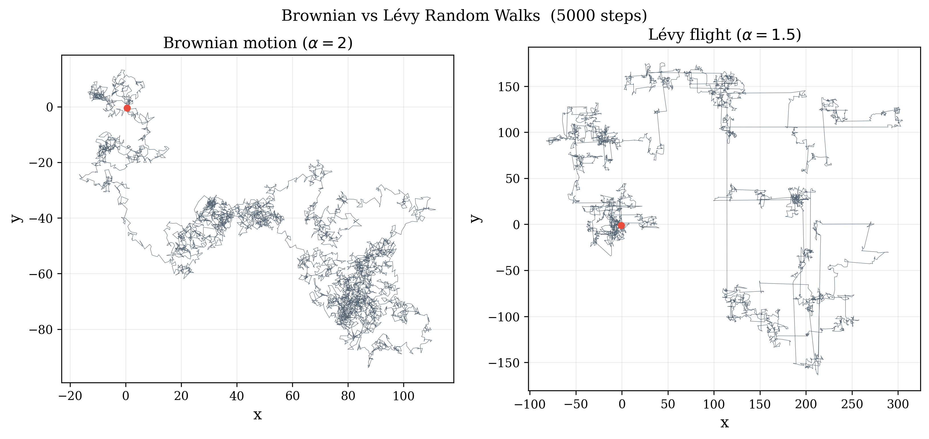
The deeper issue is that turbulent transport does not need to satisfy the assumptions behind ordinary diffusion. In a Brownian picture, the underlying random walk has a finite characteristic waiting time and a finite jump variance. In a continuous-time random walk (CTRW), if the waiting-time distribution $\psi(\tau)$ or jump distribution $\lambda(\zeta)$ develops a heavy tail,

$$\psi(\tau)\sim \tau^{-(1+\beta)}, \qquad \lambda(\zeta)\sim |\zeta|^{-(1+\alpha)},$$

with $0<\beta<1$ and $0<\alpha<2$, then long trapping events and large jumps remain important at large scales [5, 6]. In that case the standard central limit theorem no longer gives ordinary Gaussian diffusion. This is the setting in which one speaks of anomalous transport, memory effects, and, when the jump distribution is heavy-tailed, Lévy-flight-type behavior as seen in 1.

This is relevant in plasma turbulence. Del-Castillo-Negrete, Carreras, and Lynch studied tracer transport in pressure-gradient-driven plasma turbulence and found non-Gaussian radial-displacement probability density functions (pdfs) with algebraic tails together with superdiffusive scaling of moments [4]. In physical terms, turbulent eddies can trap tracers for long times, while avalanche-like events can produce large radial flights. That result does not by itself determine what diagnostic should be used on experimental signals, but it does show that Gaussian, local, and purely linear assumptions are not guaranteed.

Recent experiments also point to coupling across scales. In HL-2A, a rotating $m/n=2/1$ tearing mode was found to modulate local perpendicular flow and turbulence, and the modulation of density fluctuations extended beyond the island region toward the edge. The edge particle flux was also affected [7]. Results of this kind suggest that fluctuation measurements at two locations may reflect more than a simple local phase delay. One therefore wants diagnostics that can address nonlinear dependence and directionality.

The usual starting point for comparing two signals $x(t)$ and $y(t)$ is the linear cross-correlation

$$C_{xy}(\tau)= \frac{\langle x(t)y(t+\tau)\rangle} {\sqrt{\langle x^2\rangle\langle y^2\rangle}},$$

where $\tau$ is the time lag and $\langle \cdot \rangle$ denotes a time average. This is useful for phase propagation and coherence, but it has clear limits in broadband turbulence. As emphasized by Ding et al., vanishing linear correlation does not imply independence unless the statistics are Gaussian, deformation of the waveform can shorten the apparent linear correlation length, and the standard correlator gives no direct directional measure of nonlinear coupling [1]. These are the reasons for going beyond linear analysis here.

The main method in this report is the nonlinear conditional cross-correlation method introduced by Ding et al. for electrostatic fluctuations in STOR—M [1]. Their results indicated that the direction of fluctuation correlation reversed across the L—H transition and that the nonlinear correlation length was substantially longer than the linear one. More recently, the same method was applied to floating-potential fluctuations in TJ-II, where the reported propagation direction changed from outward without biasing to inward with negative biasing [8]. The secondary method is transfer entropy, an information-theoretic measure of directional dependence that has been used by van Milligen and collaborators to study both turbulence coupling and radial heat propagation [2, 9]. The two methods are different in construction, so comparing them is useful.

This report first sets out the mathematical form of Non=linear Cross Correlation (NLCC) and Transfer Entropy (TE). The algorithms are validated against well know differential equations with know coupling strengths and later applied plasma fluctuation data from experiments. The discussion of anomalous transport is included only to motivate why linear correlation alone is not enough.

Nonlinear directional diagnostics

Nonlinear conditional cross-correlation

The NLCC method begins by reconstructing local dynamics from scalar signals. Given two discrete signals $x_i=x(t_i)$ and $y_i=y(t_i)$ sampled at a common time step $\Delta t$, define the delay vectors

$$X_i^{(M)}=\frac{1}{\sqrt{M}}\left(x_i,x_{i+m},\dots,x_{i+(M-1)m}\right), \qquad Y_i^{(M)}=\frac{1}{\sqrt{M}}\left(y_i,y_{i+m},\dots,y_{i+(M-1)m}\right),$$

where $m$ is the delay in samples and $M$ is the embedding dimension [1, 8]. If the two signals are dynamically related, then neighborhoods in the reconstructed $X$-space should constrain neighborhoods in the reconstructed $Y$-space.

This is measured by the conditional dispersion

$$\sigma_{xy}^{(M)}(\varepsilon)= \left[ \frac{ \sum_{i\ne j}\left|Y_i^{(M)}-Y_j^{(M)}\right|^2 H\!\left(\varepsilon-\left|X_i^{(M)}-X_j^{(M)}\right|\right)} {\sum_{i\ne j}H\!\left(\varepsilon-\left|X_i^{(M)}-X_j^{(M)}\right|\right)} \right]^{1/2},$$

where $\varepsilon$ is a scale parameter and $H$ is the Heaviside step function [1, 8]. The quantity $\sigma_{xy}^{(M)}(\varepsilon)$ is the measure of the of the $Y$-vectors under the condition that the corresponding $X$-vectors lie within an $\varepsilon$-ball. Exchanging $x$ and $y$ gives $\sigma_{yx}^{(M)}(\varepsilon)$.

Following Ding et al., let $\varepsilon_{90}$ satisfy

$$\sigma(\varepsilon_{90})=0.9\,\sigma_{\max},$$

where $\sigma_{\max}$ is the maximum of the dispersion curve over the scanned range for the final convergin dimension M. The nonlinear correlation coefficient is then

$$g_{xy}=\frac{\varepsilon_{90}}{\varepsilon_{\max}},$$

where $\varepsilon_{\max}$ is the maximum attractor size in the conditioning space [1]. To reduce amplitude dependence one may normalize with the corresponding auto-correlations,

$$G_{xy}=\frac{g_{xy}}{\sqrt{g_{xx}g_{yy}}}.$$

Directionality enters because, in general, $g_{xy}\neq g_{yx}$. In this report the asymmetry is written as

$$S_{xy}=\frac{g_{xy}-g_{yx}}{g_{xy}+g_{yx}}.$$

With this convention, $S_{xy}>0$ indicates stronger directed coupling from $x$ to $y$, while $S_{xy}<0$ indicates the reverse. This sign convention is stated explicitly because the original Ding paper is known to contain a sign typo in the asymmetry formula [1].

NLCC is therefore a geometric measure. It does not compare the two signals by linear waveform similarity. Instead, it asks whether neighborhoods in one reconstructed dynamics constrain neighborhoods in the other. For that reason, it is better suited than ordinary cross-correlation for nonlinear directional coupling.

Transfer entropy

Transfer entropy approaches the same problem from an information-theoretic side. For two processes $X$ and $Y$, the transfer entropy from $Y$ to $X$ is

$$T_{Y\to X} = \sum p(x_{n+1},x_n^{(k)},y_n^{(l)}) \log_2 \frac{p(x_{n+1}\mid x_n^{(k)},y_n^{(l)})} {p(x_{n+1}\mid x_n^{(k)})},$$

where $x_n^{(k)}$ and $y_n^{(l)}$ are histories of lengths $k$ and $l$ [2, 10]. Here $p$ denotes the relevant probability distribution. If the past of $Y$ adds no predictive information beyond the past of $X$, then $T_{Y\to X}=0$.

Using conditional probabilities, the same quantity may be written as

$$T_{Y\to X} = \sum p(x_{n+1},x_n^{(k)},y_n^{(l)}) \log_2 \frac{ p(x_{n+1},x_n^{(k)},y_n^{(l)})\,p(x_n^{(k)})} {p(x_n^{(k)},y_n^{(l)})\,p(x_{n+1},x_n^{(k)})}.$$

This makes clear that TE is a conditional mutual-information measure [2]. Since in general $T_{Y\to X}\neq T_{X\to Y}$, it is directional by construction.

In plasma applications the available stationary windows are often short, so the probability distributions must be estimated with coarse graining. In practice this means a small number of bins and short histories, often $k=l=1$ [2]. The delay is then chosen using the signal period, decorrelation time, or self-mutual information. In this simplified form TE has been used in two ways relevant here. First, it has been used to study directional coupling between turbulence-related quantities near confinement transitions [2]. Second, it has been used to study radial heat propagation, where the analysis suggested minor transport barriers, “jumping” propagation, and competing fast and slow channels [9].

For the present report, TE is not a replacement for NLCC. NLCC measures conditional geometry in reconstructed phase space. TE measures conditional reduction of uncertainty. The two methods probe related but different features of coupled dynamics.

Validation on synthetic Van der Pol and predator—prey models

Before applying NLCC and transfer entropy (TE) to experimental probe signals, both methods were tested on synthetic systems with prescribed coupling. The aim is to verify that the implementations recover the imposed direction on a common analysis setup and to record the cases in which the two diagnostics do not agree. $S_{xy}>0$ denotes stronger influence from $x$ to $y$, while $S_{xy}<0$ denotes the reverse. The synthetic benchmarks were analyzed with a shared window length $N=1200$, NLCC parameters $\tau=1$, $M=2$, $d_M=2$, $\log_2\epsilon\in[-4,1]$ sampled at 16 points, and TE parameters given by one-step prediction with coarse-grained histograms. The sliding-window scans below use a step of 300 samples. These common settings were chosen to compare the two methods directly rather than retuning each case separately.

Coupled Van der Pol oscillators

The first benchmark family is the coupled Van der Pol system used by Ding et al. for the original NLCC validation [1]:

$$\begin{aligned} \ddot{x} &= \left[a_1-(x+b y)^2\right]\dot{x}-(x+b y), \\ \ddot{y} &= \left[a_2-(y+a x)^2\right]\dot{y}-(y+a x). \end{aligned}$$

Here $x(t)$ and $y(t)$ are the oscillator amplitudes, $a_1$ and $a_2$ control the self-excitation of the two oscillators, and $a$ and $b$ determine the coupling direction from y to x. Ding et al. integrated this system with time step $\Delta t=0.01$ and showed that the nonlinear coefficients $g_{xy}$ and $g_{yx}$ saturate with embedding dimension; they also reported that the method remains usable under moderate added Gaussian noise [1]. Two Ding-type cases were used as direct reversal tests. In Case 1, $(a_1,a_2,a,b)=(1,1,2.5,0)$, so the imposed direction is $x\to y$. In Case 2, $(a_1,a_2,a,b)=(1,1,0,2.5)$, so the imposed direction is $y\to x$. Representative time traces are shown in Fig. 2. For Case 1, NLCC gives

$$G_{xy}=0.931,\qquad G_{yx}=0.722,\qquad S_{xy}=+0.127,$$

and TE gives

$$\mathbf{T}_{\mathrm{VDP},1}= \begin{pmatrix} 0 & 0.129\\ 0.115 & 0 \end{pmatrix},$$

so both methods identify $x\to y$. For Case 2, the ordering reverses,

$$G_{xy}=0.728,\qquad G_{yx}=0.952,\qquad S_{xy}=-0.133,$$

with

$$\mathbf{T}_{\mathrm{VDP},2}= \begin{pmatrix} 0 & 0.113\\ 0.127 & 0 \end{pmatrix},$$

so both methods identify $y\to x$. This reproduces the directional reversal expected from the coupling coefficients and matches the behaviour reported by Ding et al. for the original NLCC algorithm [1].

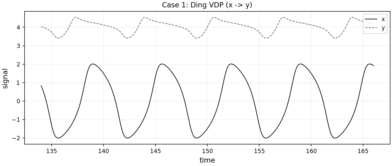
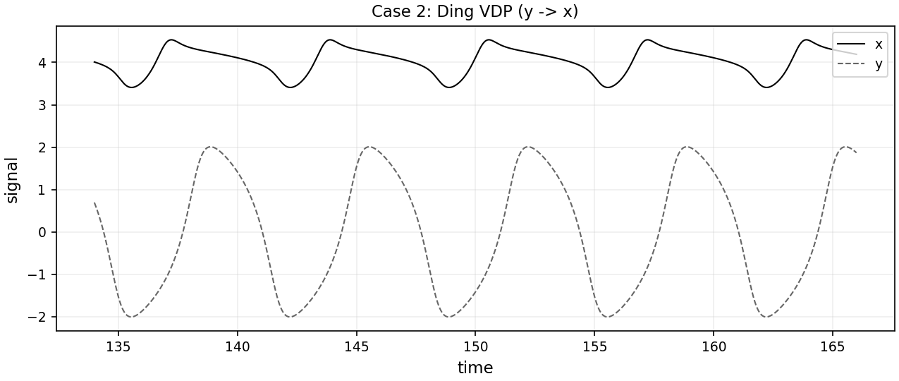
Synthetic time series for the Ding-type coupled Van der Pol system under reversal of the imposed drive direction.

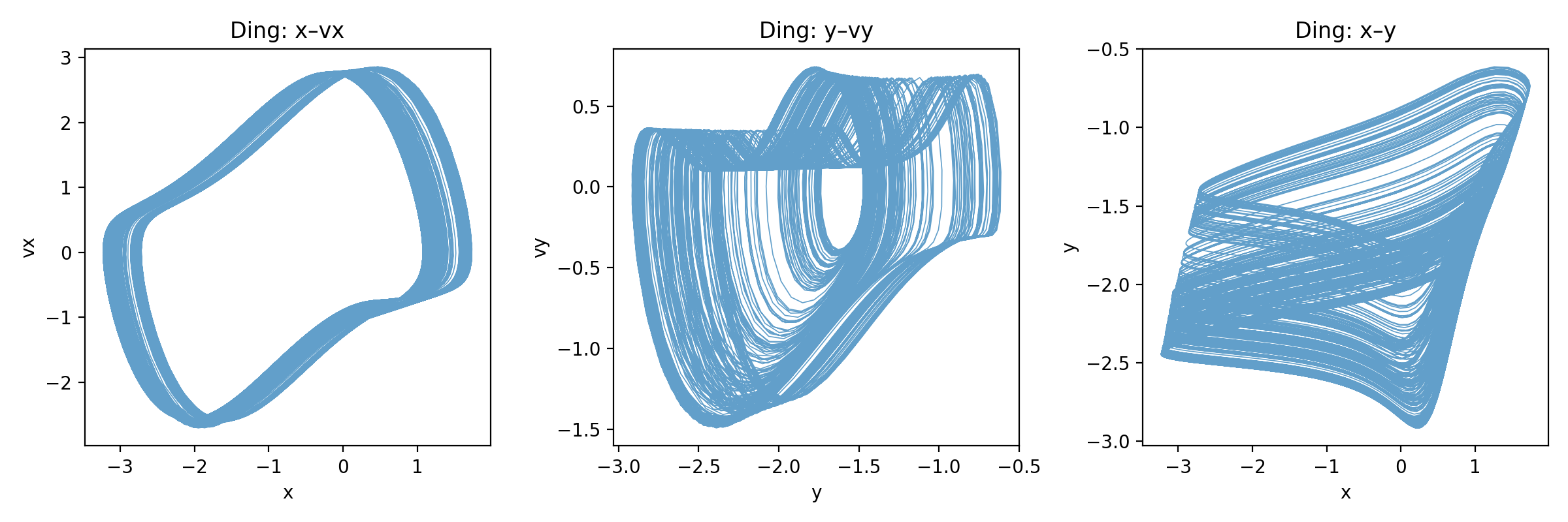
The corresponding phase portraits for the Ding regime are shown in Fig. 3. In the $(x,\dot{x})$ plane the trajectory fills a thick closed band rather than a thin limit cycle. The $(y,\dot{y})$ plane is more distorted, and the $(x,y)$ projection occupies a broad slanted ribbon. These are the geometric features expected of the strongly nonlinear regime emphasized by Ding et al., where the attractor is not close to a single smooth closed orbit [1]. In this regime the directional ordering is recovered by both NLCC and TE on the shared short-window analysis.

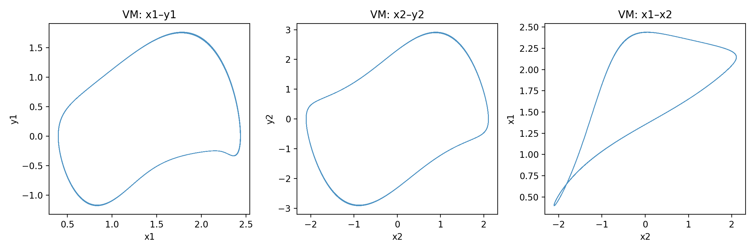
A third Van der Pol case was retained in the weakly detuned van Milligen regime. Van Milligen et al. use the first-order form

$$\begin{aligned} \dot{x}_i &= y_i, \\ \dot{y}_i &= \left[\varepsilon_i-\left(x_i+\sum_j \kappa_{ij}x_j\right)^2\right]y_i -\left(x_i+\sum_j \kappa_{ij}x_j\right), \end{aligned}$$

and for the two-oscillator validation take $\varepsilon=(1,1.1)$ with

$$\kappa= \begin{pmatrix} 0 & 1\\ 0 & 0 \end{pmatrix},$$

so that oscillator 2 drives oscillator 1 [2]. They analyze this case with coarse graining and show that the dominant information flow is correctly recovered in their TE framework [2]. In the present short-window comparison, the corresponding synthetic case gives

$$G_{xy}=0.837,\qquad G_{yx}=0.966,\qquad S_{xy}=-0.071,$$

while the TE matrix is

$$\mathbf{T}_{\mathrm{VDP},3}= \begin{pmatrix} 0 & 0.147\\ 0.083 & 0 \end{pmatrix}.$$

Thus NLCC identifies $y\to x$, while TE identifies $x\to y$ on this shared configuration.

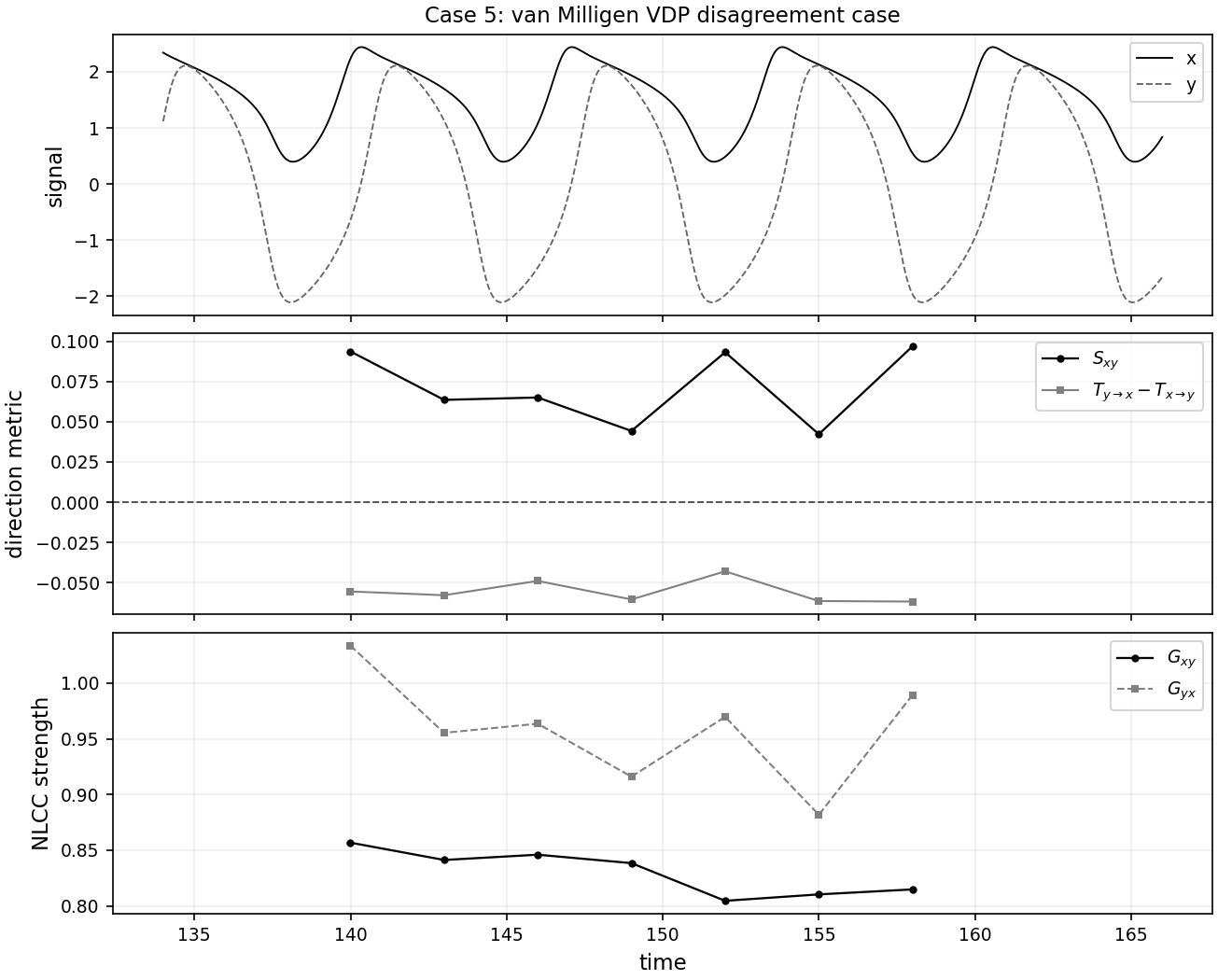
The phase portraits in Fig. 4 show why this case is geometrically different from the Ding regime. Both single-oscillator projections lie close to thin closed curves, and the $(x_1,x_2)$ projection traces a narrow loop. This is much closer to a quasi-periodic near-phase-locked state than to the broadened Ding attractor. In the midterm TE benchmark, the van Milligen asymmetry was already much smaller than in the Ding regime and became sensitive to window size once $N$ increased, whereas the NLCC asymmetry remained correctly signed [2]. The same qualitative feature is retained here: the weakly detuned benchmark is the case in which TE is more estimator-sensitive.

The window-by-window evolution for this disagreement case is shown in Fig. 5. In the shared short-window scan, the NLCC metric keeps one sign throughout, while the TE difference keeps the opposite sign throughout. This case is therefore kept as part of the benchmark set.

Predator—prey model

The second benchmark family is the reduced predator—prey model used by van Milligen et al. to study the interaction between turbulence level, zonal-flow shear, and mean shear [2]:

$$\begin{aligned} \frac{dE}{dt} &= \left(\frac{1}{1+V'^2+U'^2}-E\right)E, \\ \frac{dV'}{dt} &= \left(aE^2+cU'^2-b\right)V', \\ \frac{dU'}{dt} &= \left(\frac{aE^2}{1+V'^2}-b\right)U' + dE^2V'. \end{aligned}$$

Here $E$ denotes turbulence amplitude, $U'$ zonal-flow shear, and $V'$ mean-flow shear. Van Milligen et al. simulated this system with parameters

$$a=0.204,\qquad b=0.16,\qquad c=0.714,\qquad d=0.5,$$

reported a mean oscillation period of about $40$ samples, and obtained the resultant coupling strength is embedded in the $3 \times 3$ transfer matrix. The net strength to one oscillator (physical quantities) from the other two can be summed up from the relevant matrix element.

$$\mathbf{T}_{\mathrm{pp}}= \begin{pmatrix} 0 & 0.4913 & 1.0791\\ 0.6320 & 0 & 0.8540\\ 0.7084 & 1.0809 & 0 \end{pmatrix},$$

which gives a directed interaction graph among the three variables [2]. In the present work, two projected pairs from the same trajectory were used so that they could be compared on the same two-signal NLCC and TE pipeline as the Van der Pol data.

For the pair $(E,V')$,

$$G_{xy}=0.723,\qquad G_{yx}=0.697,\qquad S_{xy}=+0.019,$$

and

$$\mathbf{T}_{E,V'}= \begin{pmatrix} 0 & 0.647\\ 0.556 & 0 \end{pmatrix}.$$

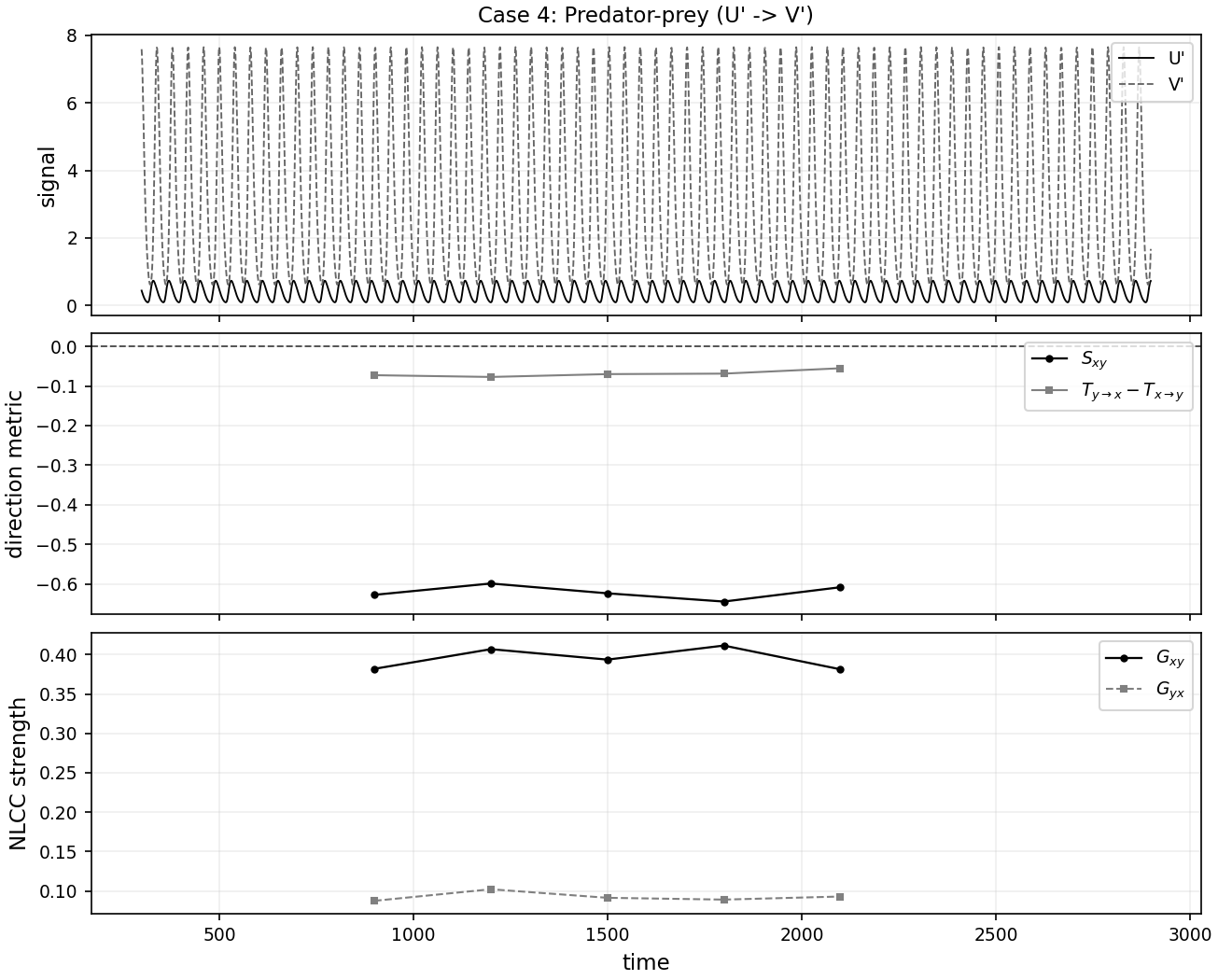
Both methods identify $E\to V'$. For the pair $(U',V')$,

$$G_{xy}=0.400,\qquad G_{yx}=0.094,\qquad S_{xy}=+0.620,$$

and

$$\mathbf{T}_{U',V'}= \begin{pmatrix} 0 & 0.905\\ 0.832 & 0 \end{pmatrix}.$$

Again both methods identify the same direction, now $U'\to V'$. The sliding-window scan for this second pair is shown in Fig. 6. In the synthetic package, this is the clearest agreement case: the NLCC sign, the TE sign, and their window-by-window agreement all remain stable across the scan.

On the shared analysis setup, the synthetic results give four agreement cases and one disagreement case. The two Ding-type reversals show that both methods respond correctly when the imposed coupling is reversed. The two predator—prey projections show that the same reduced transport model can yield both modest and strong directional asymmetry depending on the observable pair. The van Milligen benchmark is the weak-asymmetry case in which TE becomes more sensitive to estimator choices than NLCC.

Application to SWIP data

SWIP discharge and measurement geometry

The final experimental test case in this thesis is the SWIP data set from HL-2A shot #36656. This discharge was analyzed by Jiang et al. in NBI-heated L-mode plasmas and was characterized by a naturally rotating $m/n=2/1$ tearing mode. The reported plasma current was approximately $I_p \approx 160\,\mathrm{kA}$, the line-averaged density was $\bar n_e \approx 1.1\times 10^{19}\,\mathrm{m}^{-3}$, and the neutral beam power was ramped in two steps, first to $250\,\mathrm{kW}$ and then to $500\,\mathrm{kW}$. The island center was located near $R\approx 193\,\mathrm{cm}$, close to the $q=2$ surface, and the island width decreased from about $8\,\mathrm{cm}$ before NBI to about $5\,\mathrm{cm}$ at $500\,\mathrm{kW}$. Jiang et al. further reported that the local perpendicular flow and turbulence level were modulated by the island rotation, that the modulation of density fluctuations extended beyond the island region toward the edge, and that the particle flux near the strike point was affected. These observations make shot #36656 a useful final test case for nonlinear directional diagnostics, because it is already known to contain coupled MHD activity, flow modulation, and fluctuation response. [7]

The diagnostic layout is important for interpreting the results. Electron cyclotron emission and electron cyclotron emission imaging were used by Jiang et al. to follow the electron-temperature structure and rotating island. Doppler backscattering measured perpendicular flow and short-scale density fluctuations, while beam emission spectroscopy measured longer-wavelength density fluctuations over a radial interval near the midplane. Mirnov coils identified the $m/n=2/1$ mode. The analysis here uses the BES channels, so it should be understood as a fluctuation-coupling analysis within the measurement region rather than a direct reconstruction of the full island dynamics. [7]

Figure 7 shows the approximate BES channel locations used in the present analysis. This figure is included to show the spatial relation between the specific channel pairs and reference channels discussed below.

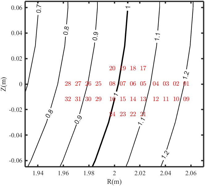
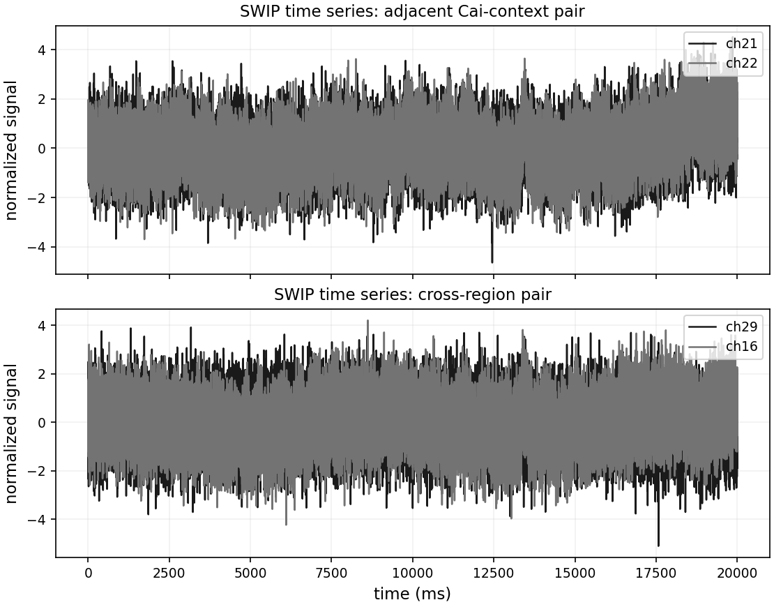
Figure 8 shows representative normalized time series for two channel pairs used below: the adjacent Cai-context pair 21—22 and the pair 29—16, corresponding to distinct regions in the tokamak, indicated by 7. In both cases the signals are broadband and intermittent, with no single persistent phase relation visible over the full $20\,\mathrm{s}$ record. This is the kind of setting in which ordinary linear cross-correlation can become difficult to interpret. Ding et al. emphasized that linear correlation does not distinguish nonlinear dependence from independence when the statistics are non-Gaussian, and that it does not provide a directional measure of nonlinear coupling. This motivates the application of NLCC and transfer entropy to the SWIP signals. [1]

NLCC on SWIP channel pairs

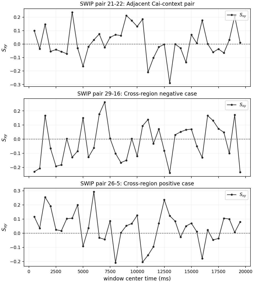
The NLCC results are summarized in Fig. 9. For the adjacent pair 21—22, the asymmetry $S_{xy}$ changes sign several times across the discharge. There are broad positive intervals in the middle part of the record and sharper negative excursions later. This pair is therefore not well described by one fixed direction over the full time interval.

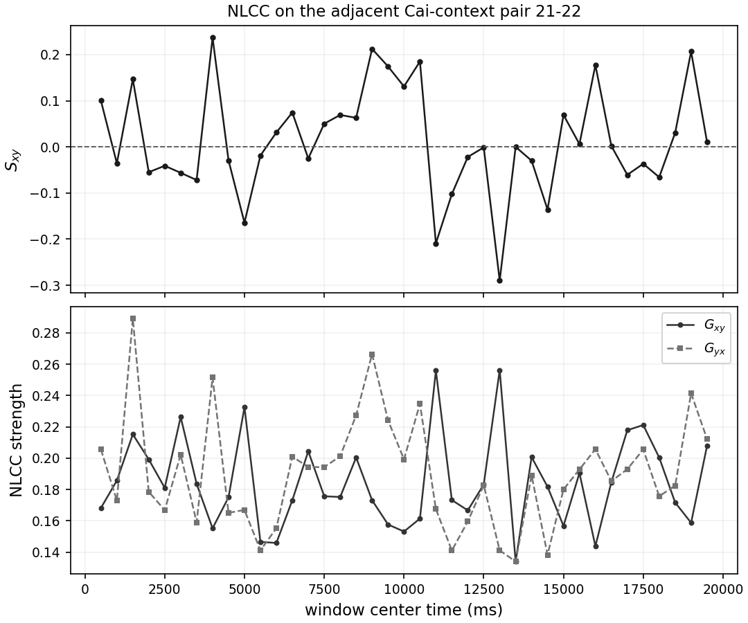
This is clearer in Fig. 10, where the asymmetry $S_{xy}$ is shown together with the normalized nonlinear strengths $G_{xy}$ and $G_{yx}$. The two strengths remain of comparable magnitude for much of the record, while the asymmetry changes more strongly. The important point is therefore not simply that the pair alternates between coupled and uncoupled states. Rather, the nonlinear coupling strengths remain of similar order while the directional balance between the two channels varies in time. This is the main value of NLCC in the SWIP data: it resolves a time-dependent pairwise asymmetry that is not obvious from the raw waveforms.

The cross-region pair 29—16 shows a different but related behavior. Its $S_{xy}$ curve is more often negative than positive, but sign reversals are still present. It is therefore safer to describe this pair as having a negative tendency rather than a fixed negative direction. Pair 26—5 acts as the opposite case: positive intervals are broader and more frequent than negative ones. The three examples in Fig. 9 do not support a single global propagation direction for the entire discharge. They show that different channel pairs can have different preferred signs, and even within one pair the asymmetry may reverse in time.

This also fits earlier NLCC work on plasma fluctuations. Ding et al. introduced the method because conventional correlators can miss nonlinear dependence and cannot assign a directional asymmetry. In STOR—M they found that the direction of the fluctuation correlation reversed across the L—H transition, and that the nonlinear correlation length was substantially longer than the linear one. [1] More recently, Bsharat et al. applied the same conditional-dispersion framework to TJ-II and reported a change from outward propagation without biasing to inward propagation under negative biasing. [8] The SWIP results are less clean than those cases, but they are consistent with the same general point: NLCC is useful here as a time-resolved measure of directional asymmetry between specific pairs.

Transfer entropy with fixed reference channels

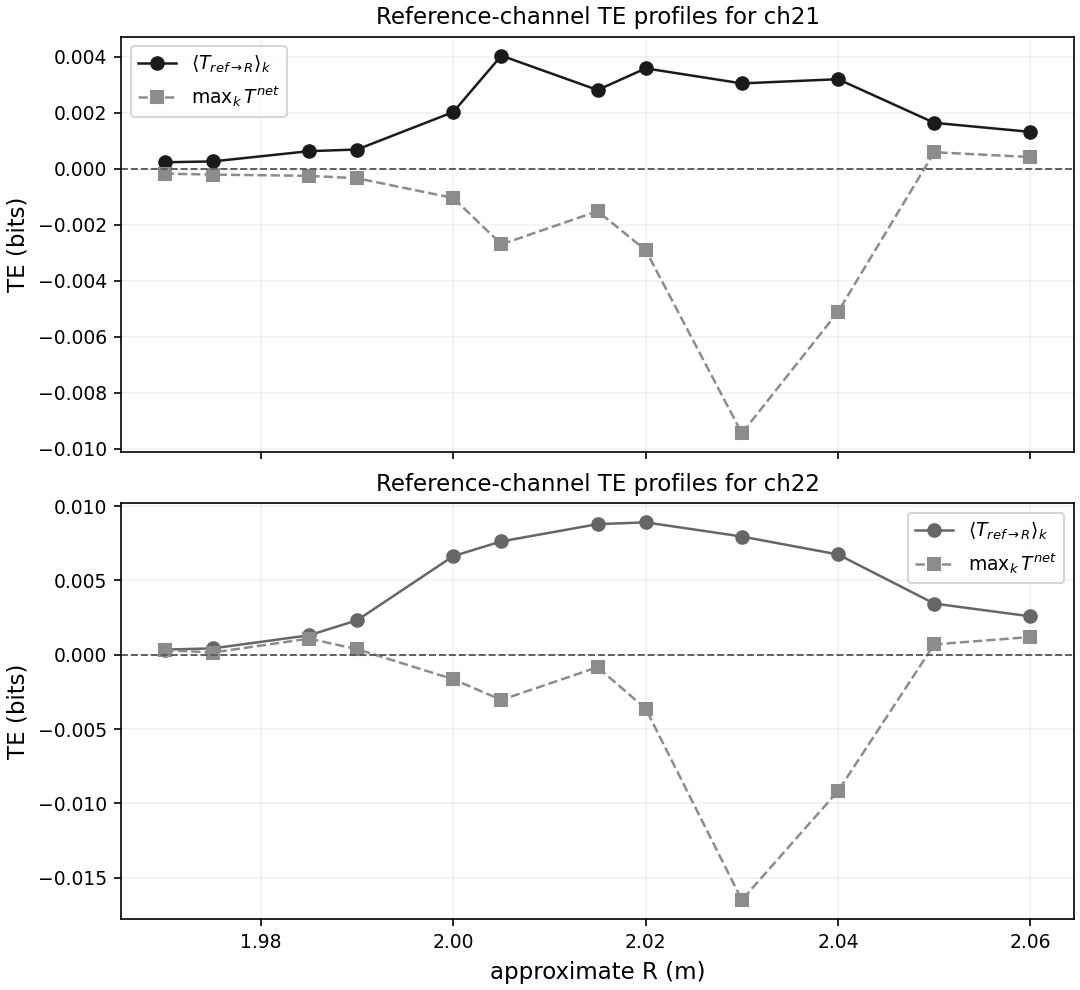
The TE results are organized around fixed reference channels and are shown in Fig. 11. For both reference channels 21 and 22, the mean directed TE is not spatially flat. It rises from the inner side of the reconstructed radial interval, reaches a maximum in the middle, and then decreases again farther out. The net TE is more selective than the mean directed TE. Its strongest negative feature is concentrated near $R\approx 2.03\,\mathrm{m}$, especially for reference channel 22. This suggests that the directional imbalance is localized in a restricted radial region rather than spread uniformly across the BES array.

This interpretation is consistent with the way transfer entropy has been used in the fusion literature. Van Milligen et al. define TE as a directional conditional mutual-information measure and note that practical estimation in plasma data usually requires coarse graining and short effective histories because stationary records are limited in length. [2] In later radial heat-propagation work, van Milligen et al. used a fixed reference position and examined TE as a function of lag and position. [9] The SWIP TE curves follow this logic: the estimator is coarse grained, the reference channels are fixed, and the lag dependence is scanned rather than assuming a single preferred delay. The values in the present analysis are modest, so the result should be interpreted through the persistence of spatial structure and sign, not through the absolute magnitude of one isolated point.

Figure 12a shows that the TE structure is not a single-lag artifact. For reference channel 21, the directed TE curves maintain similar ordering across $k=1,\dots,12$, and the net TE near $R=2.03\,\mathrm{m}$ remains negative across almost the entire lag scan. By contrast, the outer curves near $R=2.05\,\mathrm{m}$ remain much closer to zero. The directional structure is therefore more dependent on region than on lag within the scanned range.

Figure 12b shows that this structure also evolves in time. The late block, $15$—$20\,\mathrm{s}$, develops the strongest negative trough near $R\approx 2.03$—$2.04\,\mathrm{m}$, whereas the earlier blocks are flatter and remain closer to zero. This makes the TE result time-dependent in the same broad sense as the NLCC analysis.

A comparison with earlier TE work is also possible. In their study of radial heat propagation, van Milligen et al. reported non-flat TE structures associated with localized transport features, minor barriers, and occasional apparent jumps over intermediate radii. [9] The present SWIP measurements are different in both diagnostic and observable, so that full transport picture should not be imported directly. Still, the comparison is useful at a limited level: a spatially nonuniform TE profile is not unusual in strongly nonlinear plasma data, and a localized directional feature is more plausible than a uniform monotone radial trend.

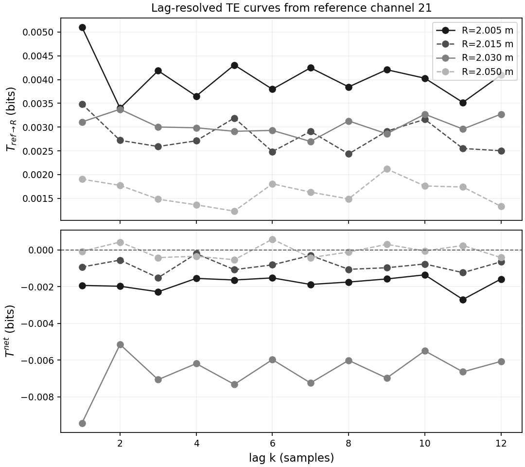
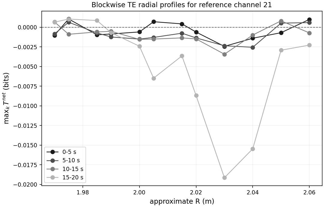
Additional TE structure from reference channel 21. Top: the TE ordering is broadly stable across the lag scan, and the strongest negative net TE remains concentrated near R ≈ 2.03 m. Bottom: the same spatial region becomes more pronounced in the late 15–20 s block, while earlier blocks remain flatter.

Interpretation in the HL-2A context

The present nonlinear results are consistent with the experimental picture reported by Jiang et al. for shot #36656. In that study, the rotating $2/1$ island modulated local flow and micro-fluctuations, the modulation of density fluctuations extended from the island region toward the edge, and the edge particle flux was also affected. [7] Those observations support reading the present SWIP NLCC and TE results as signatures of time-dependent multiscale coupling rather than as simple two-point wave propagation.

At the same time, the claims should remain limited. The NLCC asymmetry $S_{xy}$ is a directional imbalance in conditional dispersion. Transfer entropy is a directional measure of predictive dependence. Neither one, by itself, proves a literal channel of energy transfer or a complete transport mechanism. For shot #36656, the nonlinear diagnostics do not support a single fixed global direction of interaction. Instead, they indicate two features. First, specific channel pairs exhibit intermittent asymmetry that can reverse sign in time. Second, the TE analysis from fixed reference channels reveals a broader directional structure that is localized in radius and becomes more pronounced late in the discharge.

Conclusion of the SWIP application

The SWIP results fit the picture developed in the previous sections. In the synthetic tests, NLCC and TE recovered imposed directionality in controlled nonlinear systems, while TE was more estimator-sensitive in weak-asymmetry cases. In the SWIP data, neither method returns a spatially or temporally featureless result. NLCC resolves time-dependent pairwise asymmetry, while TE reveals a more spatially organized directional structure from fixed reference channels. Overall, these results support a limited conclusion: in shot #36656, directional coupling is present, but it is neither spatially uniform nor temporally stationary. This is consistent with the broader HL-2A picture of tearing-mode modulation of flows, turbulence, and edge response. [1, 2, 7—9]